0. 前言

Reference: 8.11-8.14

下面我们再来看一个跟 Graph 有关的经典问题：The Knight’s Tour Problem.

这是一个在棋盘上的解密游戏，棋盘是 8x8 的规格，上面只有一个棋子：Knight。

目标是：找到一个路径（tour），让这颗棋子能访问整个棋盘上的每个格子，但是每个格子只能走一次。

我们将用 Graph 来解决这个问题。

思路

首先我们需要把棋子可以走的格子用 Graph 表示出来；

然后我们再用一个 Graph Algorithm 来找到长度为 rows x columns - 1 的路径（也就是棋盘的总格数-1，每个格子访问一次）。

1. 用 Graph 表示问题

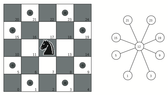
每个格子是一个 node，棋子可以走的路径是 edge。

• 我们需要用数字来代表棋盘的格子，posToNodeId function 可以完成这个工作

• 我们需要一个 helper function - genLegalMoves 来生成棋子当前可以走的路径，每个格子最多有 8 个可行路径。

代码

# pip3 install pythonds
from pythonds.graphs import Graph

def knightGraph(bdSize):
    ktGraph = Graph()
    for row in range(bdSize):
       for col in range(bdSize):
           nodeId = posToNodeId(row,col,bdSize)
           newPositions = genLegalMoves(row,col,bdSize)
           for e in newPositions:
               nid = posToNodeId(e[0],e[1],bdSize)
               ktGraph.addEdge(nodeId,nid)
    return ktGraph

def posToNodeId(row, column, board_size):
    return (row * board_size) + column
  
def genLegalMoves(x,y,bdSize):
    newMoves = []
    moveOffsets = [(-1,-2),(-1,2),(-2,-1),(-2,1),
                   ( 1,-2),( 1,2),( 2,-1),( 2,1)]
    for i in moveOffsets:
        newX = x + i[0]
        newY = y + i[1]
        if legalCoord(newX,bdSize) and \
                        legalCoord(newY,bdSize):
            newMoves.append((newX,newY))
    return newMoves

def legalCoord(x,bdSize):
    if x >= 0 and x < bdSize:
        return True
    else:
        return False

完成图

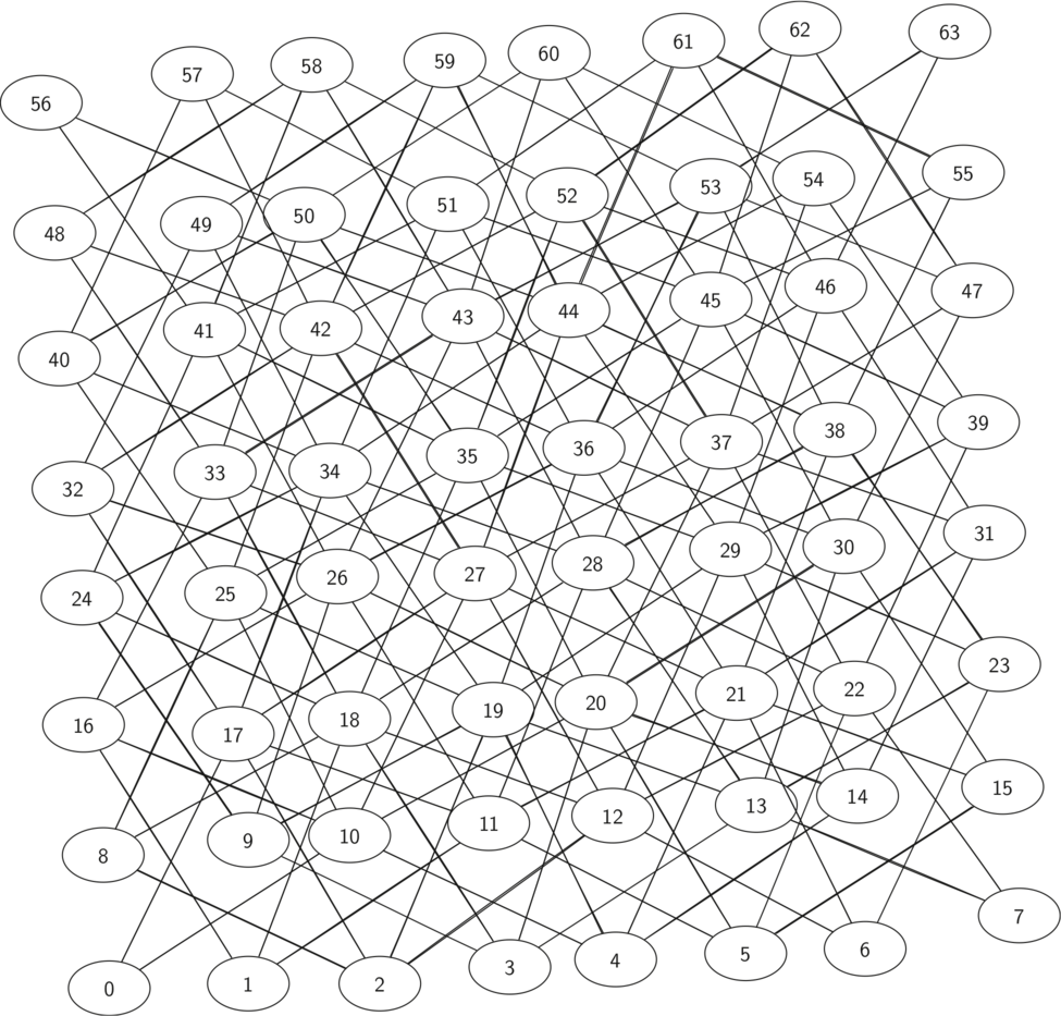
以 8x8 的棋盘为例，下图就代表了棋子所有可能的移动路径，总共是 336 个路径。

我们可以发现，在边缘位置的 node 并没有太多 edge，在中间的 node 则 edge 比较多。

Note：这个图是离散的，假如每个 node 之间都有 edge 的话，我们总共会有 4096 个 edge，但是现在这个数量（336）要少得多，邻接矩阵的填充率只有 8.2%。

2. 用 DFS 解决问题

DFS 全称是 Depth First Search，和 BFS 一样，都属于搜索算法。

DFS 和 BFS 的区别

BFS 是先访问当前 level 的所有 node，再进入下一个 level。

DFS 则是每个 node 都要搜索到底，然后才能搜下一个。当 DFS 遇到死路（没有任何可以走的路径）的时候，它会回到之前的 node，继续找寻一条可以走的路。

DFS 能让我们找到正好有 8x8-1=63 个 edge 的路径。

Whereas the breadth first search algorithm builds a search tree one level at a time, a depth first search creates a search tree by exploring one branch of the tree as deeply as possible.

两种实现

DFS 有两种实现方式：

1. 明确指出每个 node 只能经过一次，直接解决 Knight’s Tour 问题

2. 更加 general，在创建 search tree 的时候，每个 node 可以经过多次

Note: 我们在本文中会先看第一种，之后的文章中再一起学习 General 的实现方法。

3. DFS 实现 1 - 代码

knightTour 是一个递归算法，先检查 base condition，假如有了包含 64 的 edge 的路径，那么这个 function 返回 True，代表我们找到了需要的那条路径。

假如路径 < 64 那么， 我们要继续 explore 下一个 level，knightTour function 会被再一次 invoke。

颜色

DFS 也用颜色来标记哪些 node 被访问过了，颜色和 BFS 一样：

• 白色：unvisited
• 灰色：visited

死路

假如某个 node 所有的 neighbour 都被访问过了，但是还没有达到我们的目标（长度 64 的 path），那么这就是一条死路，function return False.

遇到死路怎么办？

我们要往回走（backtrack）。

怎么往回走？

在 BFS 中，我们有个 queue 来记录我们需要访问的 node；

在 DFS 中，因为我们的 function 是递归的，所以我们可以用这个隐含的 stack 来帮助我们 backtracking。

当我们遇到 False 时，我们不跳出 while loop，而是去访问当前 node 的下一个 neighbour。

# pip3 install pythonds
from pythonds.graphs import Graph, Vertex

# n： current depth in the search tree
# path: a list of vertices visited up to this point
# u: the node in the graph we wish to explore
# limit: number of nodes in the path
def knightTour(n,path,u,limit):
        u.setColor('gray')
        path.append(u)
        if n < limit:
            nbrList = list(u.getConnections())
            i = 0
            done = False
            while i < len(nbrList) and not done:
                if nbrList[i].getColor() == 'white':
                    done = knightTour(n+1, path, nbrList[i], limit)
                i = i + 1
            if not done:  # prepare to backtrack
                path.pop()
                u.setColor('white')
        else:
            done = True
        return done

图解步骤

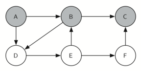
1. 从 A 开始找

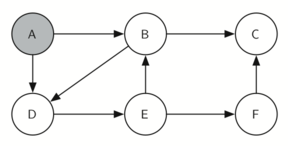
2. 来到 B，开始访问 B 的邻居们

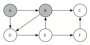
3. C 是一条死路

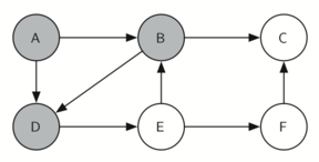
4. 回到 B

5. 访问 B 的下一个邻居 - D

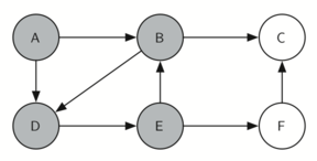
6. 更进一层，访问 E

7. 更进一层，访问 F

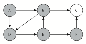
8. 完成！

找到了一条需要的路径！每个 node 都访问一次。

A -> B -> D -> E -> F -> C

4. DFS 实现 1 - 算法效率分析

算法的核心在于我们如何选择下一个要访问的 node。

我们刚才实现的算法时间复杂度是 $O(k^N)$

• k = 一个很小的常数；
• N = 棋盘上的格子数量

In particular, knightTour is very sensitive to the method you use to select the next vertex to visit.

A Search Tree for the Knight’s Tour

这个搜索树的 root 就代表 start node。

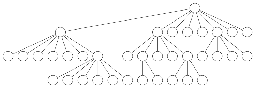
假如 start node 在棋盘的边缘，possible legal move 就比较少（只有 2），假如 start node 在中间，possible legal move 就可以达到 8，下图就代表了每个位置的 possible move。

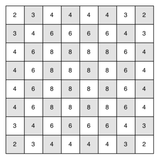
所以这个算法的搜索效率跟 start node 的位置是直接相关的。

计算

假如二叉树的高度是 N，那么 node 的总数就是 2^(N+1) - 1，那么用我们上面的例子，假如 start node 有 8 个 child node 而不是 2 个，search tree 里面 node 的总数要多很多。

由于每个 branch 的 node 数量是不确定的，我们就用一个平均值 k (an average branching factor) 来代表这个变量。

这个算法的时间复杂度是指数级的 k^(N+1) - 1。

For a board that is 5x5 the tree will be 25 levels deep, or N = 24 counting the first level as level 0.

The average branching factor is 𝑘=3.8, so the number of nodes in the search tree is 3.8^25−1 or 3.12x10^14.

For a 6x6 board, 𝑘=4.4, there are 1.5×10^23 nodes, and for a regular 8x8 chess board, 𝑘=5.25, there are 1.3×10^46.

思考：k 如何计算出来的呢？它跟棋盘的 size 有什么关系呢？

优化

resList.sort(key=lambda x: x[0]) 这行代码是关键，它保证了我们在选择下一个 node 的时候，选择 possible move 最少的那个 node。

你也可以尝试选择 possible move 最多的那个 node，来比较两种选择的效率区别。

• 只要 uncomment sort 后面的那行即可。

def orderByAvail(n):
    resList = []
    for v in n.getConnections():
        if v.getColor() == 'white':
            c = 0
            for w in v.getConnections():
                if w.getColor() == 'white':
                    c = c + 1
            resList.append((c,v))
    resList.sort(key=lambda x: x[0])
    # resList.reverse() ## select most possible move
    return [y[1] for y in resList]

为什么 most possible move 不是最优解？

因为我们可能会在棋盘中间绕圈圈，而不是走到远方。

选择 least possible move 可以让棋子尽量早点走到棋盘边缘。

This ensures that the knight will visit the hard-to-reach corners early and can use the middle squares to hop across the board only when necessary.

通过这种方式来优化算法叫做 heuristic（启发式），我们讲的这种启发式算法叫做 Warnsdorff’s algorithm，由 H. C. Warnsdorff 在 1823 年提出。

5. 结语

这篇主要讲了 DFS 搜索 Graph 的两种逻辑，以及其中一种的代码（每个 node 只能被访问一次的特殊情况），并且分析了 DFS 的时间复杂度，如何进行优化。

接下来我们会讲 DFS 搜索 Graph 的另一种情况（更加 general）。